Predicting housing price using advanced regression

Authors: He Zhang, Bingying Feng, Dingzhe Leng

Summary

Residential homes are hedonic pricing goods, whose prices are determined both by internal characteristics of the good being sold and external factors affecting it. Suppose we control the external factors, what internal features are strongly related to housing price? How good can we predict the housing price using the home features? These are the three questions that drive this project. The answers will be useful for

1. Homebuyers: For them to choose their dream house given a budget.
2. Real estate developers => choose the product to deliver
3. Real estate agents => provide valuable insights and identify the needs of customers

Data

The original data is retrieved from a Kaggle open competition. (https://www.kaggle.com/c/house-prices-advanced-regression-techniques/data) It covers data of Housing data that describes features of residential homes in Ames, Iowa sold between 2006 and 2010. There are 80 explanatory variables (23 nominal, 23 ordinal, 14 discrete, and 20 continuous) describing the homes in different aspects such as space, amenities, conditions, zoning, etc (almost every aspect of residential homes).

Method

In this project, we will build models to explain what features are related to home prices as well as models to predict home prices in Ames, Iowa.We will first conduct data cleaning, EDA and feature analysis. Then we will build Elastic net model to investigate the features that are related to home prices using methods. For the predictive models, we will incorporate more variable engineering to enhance model performance. Modern machine learning models such as Elastic net, Random Forest, Gradient Boosting and Neural Net Models will be employed in predictive modeling.

Data Analysis

EDA- Part I

Overlook

The response variable is SalePrice. There are 80 explanatory variables.

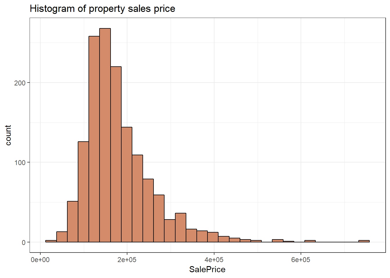
Histogram of property sales price

We created a histogram base of SalePrice and find the property sales price right-skewed. Most properties are below $200k.Given its distribution, we will later take the log of it to increase variability and approximate normality.

Data processing

Missing value

There are 34 variables with missing values. We dealt with these columns based on the data description.

We found some missing values means no such feature present such as missing value is PoolQC means no pool, missing value in MiscFeature means no such feature. So we imputed missing value in PoolQC, MiscFeature, Alley, Fence, FireplaceQu, GarageType, GarageFinish, GarageQual, GarageCond, BsmtCond, BsmtExposure, BsmtQual, BsmtFinType2, BsmtFinType1, MasVnrType and MasVnrArea as “None” or 0 meaning no such feature.

Some missing value could be imputed by geographical interpolation- taking the median value of the neighborhood such as The LotFrontage (Appendix: Box plot- lot frontage grouped by neighborhood).

Some missing value can be replaced by other values, which is reasonable to an extent. GarageYrBlt is NA if there is no garage with this property. As YearRemodAdd equals to YearBuilt if there is no remodeling, we replace the NAs in GarageYrBlt with the YearBuilt of that property.

After taking care of missing values in the previous variables, we now have only 17 variables with missing values. And these variables have only 1 or 2 missing values.

Now we impute the rest of the missing values.

MSZoning: There are 4 missing values. As RL (Residential Low density) is the most common in this data, we assign RL to the missing values.

Utilities: Only 1 property does not have all public utilities, so this is a variable of no use. We drop it.

BsmtHalfBath: 0 is the most common value, so we assign 0 to the two missing values.

Exterior1st, Exterior2nd: one observation has missing values in both cells. We assign the most common value VinylSd, VinylSd to them.

Electrical,KitchenQual,SaleType: The most common values are SBrkr, TA, WDrespectively. We assign these values to the missing value.

BsmtFullBath: We assign 0 to the missing value. We assign 0 to all other basement variables with NA as well.

Functional: The predominant value is Typ typical functionality, so we assign it to the missing values.

GarageCars,GarageArea: We assign 0 to the missing values.

So far, all missing values have been imputed.

Variable structures

We now need to make sure that all categorical and numeric variables have the correct structures. We turned MSSubClass, MoSold, YrSold into factors. OverallQual and OverallCond can be wither factor or numeric, as they are ordinal. Here we keep them as numeric for now.

str(data)
data$MSSubClass<- as.factor(data$MSSubClass)
# OverallQual and OverallCond can be wither factor or numeric, as they are ordinal. Here I keep them as numeric for now.
data$MoSold<- as.factor(data$MoSold)# Change month and year to factors
data$YrSold<- as.factor(data$YrSold)

Months & years

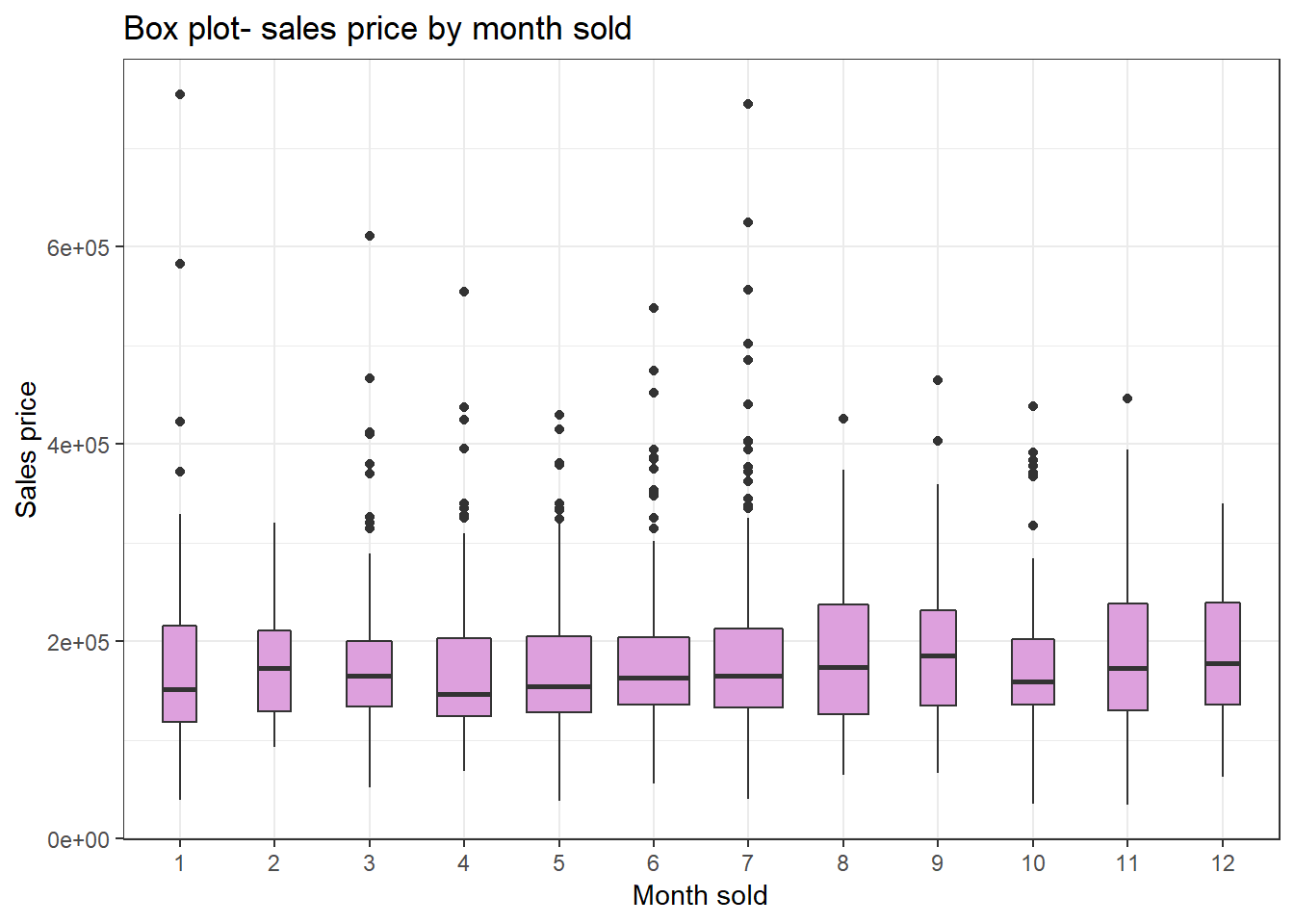Sales price by month

The gragh visualizes how sales price varies across months. We see Janurary and April have relatively low median of sale price. July has lots of outliers. Janurary and July have the highest outlier values.

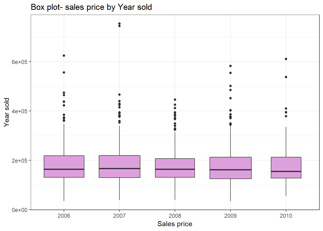Sales price by year

From this diagram, we see the price does not vary much during years. 2007 has a couple of high outlier values.

MSZoning Analysis

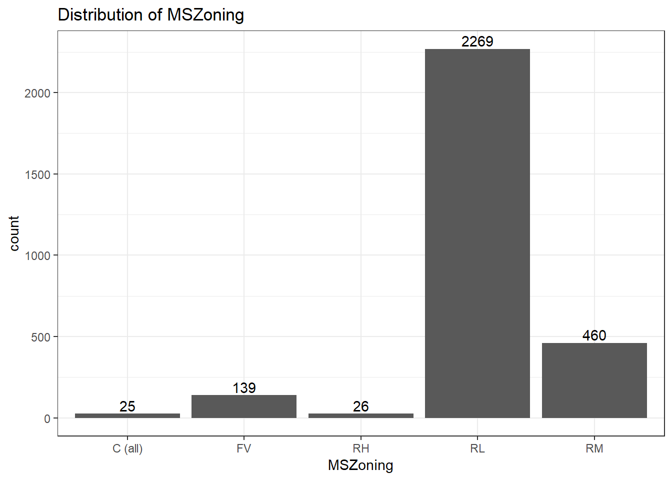Distribution of zoning

It is obvious that most of houses in this dataset are built in the area of Residential Low Density, and follows by Residential Medium Density(460 houses). Few houes are built in Commercial, Floating Village and Residential High Density.Since a large amount of houses comes to the categoreis of Residential Low Density and Residential Medium Density, these two areas should be paid more attention for housing price analysis.

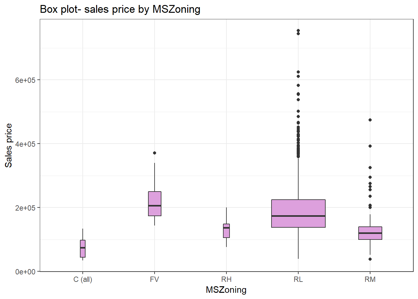Sales price by zoning

This boxplot further tells that sales price in Residential Low Density zoning has a lot of outliers, and the range is wide too. The commercial zoning has relatively low sale price.

SalePrice vs Numerical Values

We then visualized the relationship of saleprice between 4 numerical values:

• GrLivArea (Above grade (ground) living area square feet),

• TotalBsmtSF (Total square feet of basement area),

• TotRmsAbvGrd (Total rooms above grade (does not include bathrooms)),

• GarageArea (Size of garage in square feet).

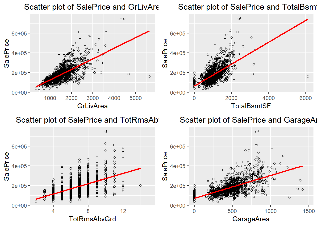Scatter plots for the four variables

All 4 variables have positive relationship with the sale price. GrLivArea and TotalBsmtSF have larger positive relationship then TotRmsAbvGrd and GarageArea.

Feature Engineering

In order to get a normalized dataset, we took the log of saleprice and deleted the original sale price column. LogSalePrice is our response variable.

Then we take ID out of our data set. We can also get the age of a house by taking Yearsold-Yearbuilt. We can also add 3 new features by the age of house. Isnew represents if a house is a new house. If the house age is 0, then mark 1 in Isnew to represent the house is a brand new one. If a house’s age is not new, but the age of the house is less then 16 years, then we mark 1 in IsRecent to represent the house is recently built. If the house is more than 50 years old, then we mark 1 in IsOld to represent the house is old.

About the neighborhood, we not only want Iowa-specific results, but also generally interpretable results. So we are generating neighborhood feature data. A next step can be adding neighborhood data from census.

Total square footage is important by intuitive. So we add a column named Totalsqft by adding GrLivArea and TotalBsmtSF.

The porch variables are not providing much variability. So we consolidate it by adding OpenPorchSF, EnclosedPorch, X3SsnPorch, ScreenPorch together. We deleted all the porch variable and only consider the consolidated one PorchArea.

For the bathroom numbers, intuitively, we count full bath as 1 and half bath as 0.5. By using the following equation, we get TotalBath= BsmtFullBath+ 0.5BsmtHalfBath+ FullBath+ 0.5HalfBath. we deleted all other bathroom variables and will only onsider the TotalBath.

Final preparation

We make two boxplot for Totalsqft and LogSalePrice to have an overview of the data. In the Totalsqft boxplot, there seems to be two very large houses, and one very small house. LogSalePrice looks fine.

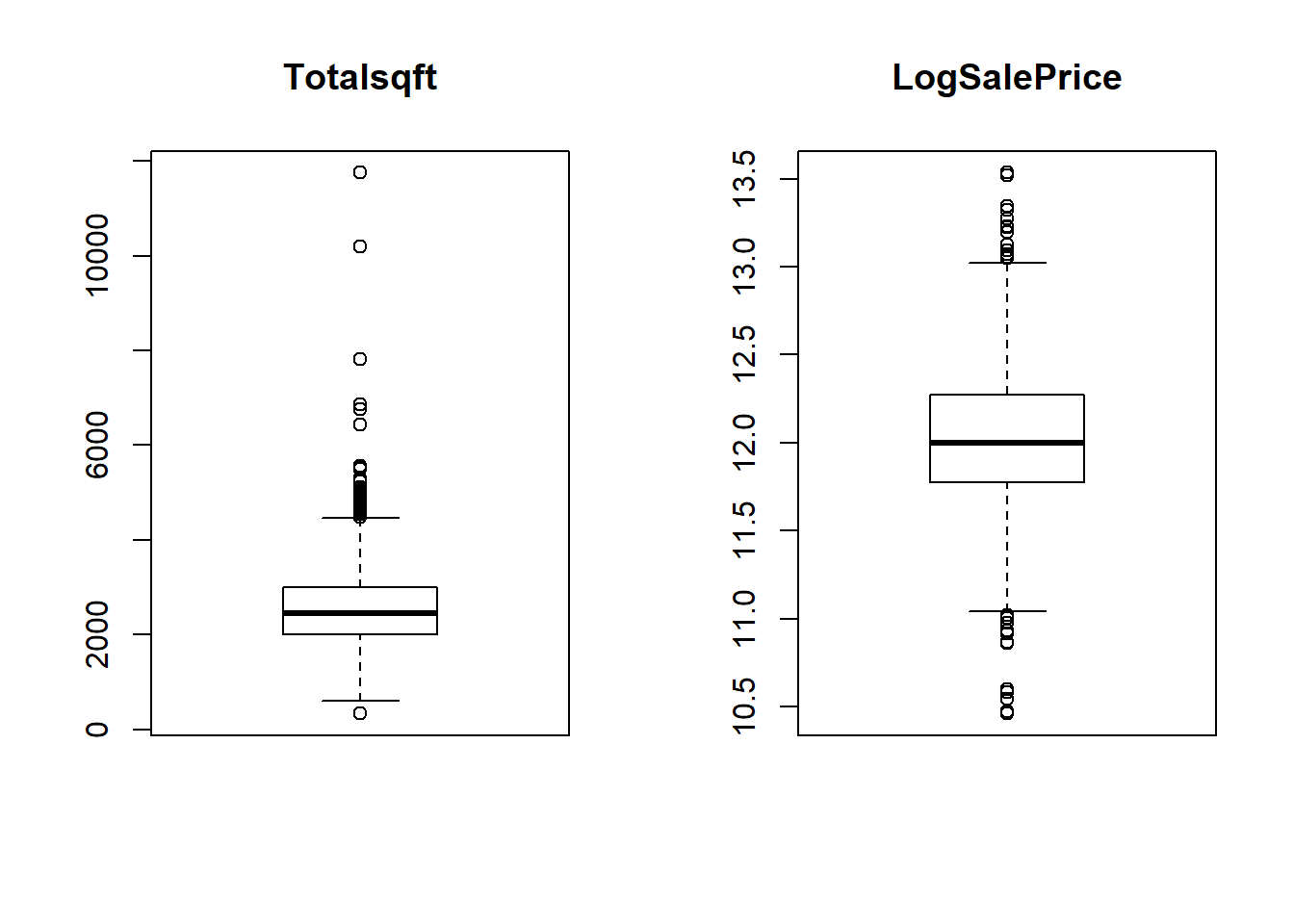Distribution of total square footage and log sale price.

Since there are many missing value in the response variable (LogSalePrice), we filtered out useful data and got our final dataset. We have 1460 observations and 79 variables and 1 response variable.

We reserve the testing data. 70% of the dataset is seperated to be training set, and the rest 30% is testing set. Now we have 1021 observations in the training set and 439 observations in the testing set.

EDA (Part II, after data processing)

Correlations

Both the correlation matrixs and heat map shows similar relationships. The top continuous variables correlated with Sale Price:

OverallQual 0.817184418

Totalsqft 0.773276841

GrLivArea 0.700926653

GarageCars 0.680624807

TotalBath 0.673010594

GarageArea 0.650887556

TotalBsmtSF 0.612133975

cor<- correlation(data)
plot(cor)

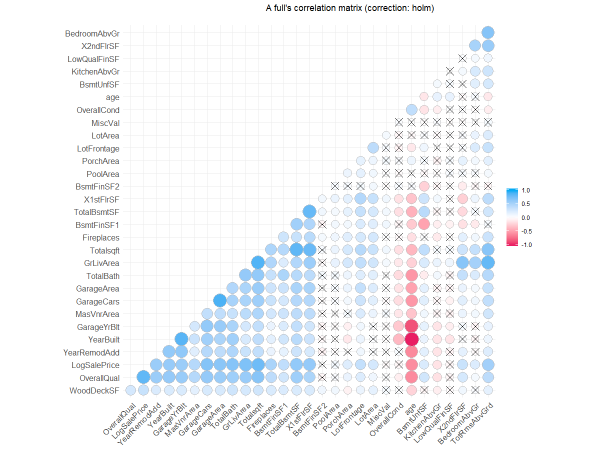Correlation matrix of continuous variables

plotData<- data%>%filter(!is.na(LogSalePrice))
plotData <-melt(cor(plotData[sapply(data, is.numeric)]))
ggplot(plotData ,
    aes(x = Var1, y = Var2, fill =value)) +
    geom_tile() +
    ylab("") +
    xlab("") +
scale_x_discrete(limits = rev(levels(plotData $Var2))) + #Flip the x- or y-axis
    scale_fill_gradient( low = "#56B1F7", high = "#132B43") +    
       guides(fill = guide_legend(title = "Correlation"))+
  theme(axis.text.x = element_text(angle=45))

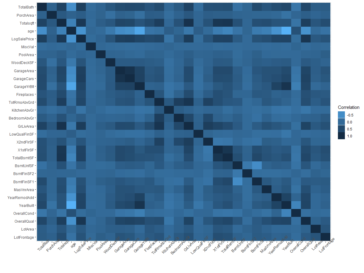Correlation heatmap of continuous variables

Models

Random Forest Modeling

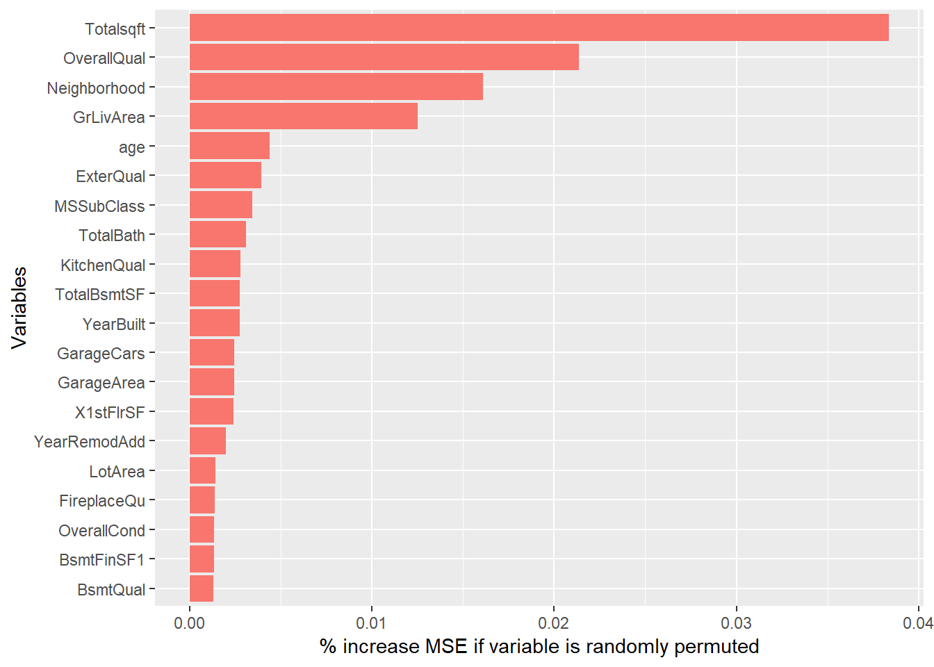
Before building the random forest model, we used the importance of random forest to see the important variables. This complements correlation analysis shows the top five important variables are Totalsqft, OverallQual, GrLivArea, Neighborhood,age which is similar to the elastic net model analysis.

data1 <- data[!is.na(data$LogSalePrice),]
eda.rf<- randomForest(LogSalePrice~., data1, mtry=25, ntree=500,importance=TRUE)
imp_RF <- data.frame(eda.rf$importance)
imp_RF <- imp_RF[order(imp_RF$X.IncMSE, decreasing = TRUE),]
setDT(imp_RF, keep.rownames = TRUE)[]

ggplot(imp_RF[1:20,], aes(x=reorder(rn, X.IncMSE),y=X.IncMSE,fill="#D48B6A")) + 
  geom_bar(stat = 'identity') + labs(x = 'Variables', y= '% increase MSE if variable is randomly permuted') + coord_flip() + theme(legend.position="none")

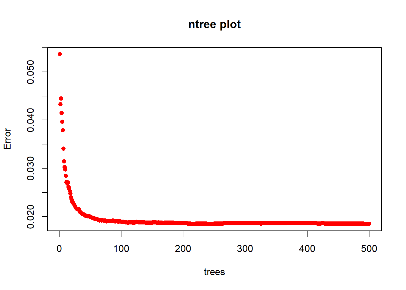
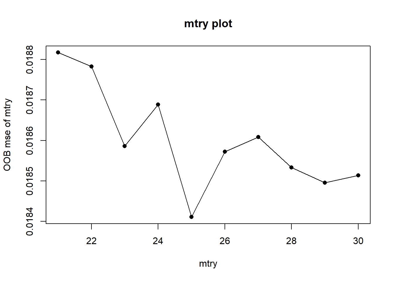
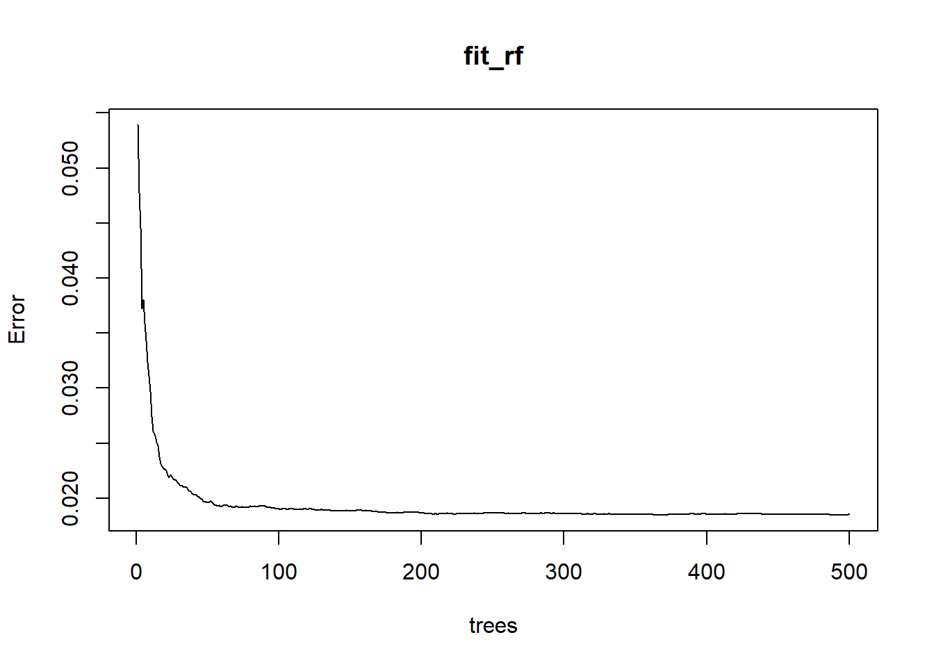
We used the training data set to build our random forest model using randomForest() functiom. We tune ntree and mtry, the two parameters of random forest.From the error ntree plot, we may need at least 100 trees to settle the OOB testing errors, so 500 trees are enough here. Now we fix ntree=500, We only want to compare the OOB mse[500] to see the mtry effects. Here we loopmtry from 1 to 30 and return the testing OOB errors.

The recommended mtry for reg trees are mtry=p/3=76/3 about 25 or 26. We run a loop around this recommended value and found smallest OOB mse at mtry= 25. We take mtry=25.

The OOB error is 0.003064511 and the testing error is 0.0219367 Testing error is smaller than the training errir, but the testing error is also relatively small. So, this model predicts the testing dataset well. The following plot shows the error based on tree numbers.

Boosting tree

After trying different tuning parameter, we get n.trees = 20000, interaction.depth = 2, cv.folds = 5 for minimizing the training error.

fit_boosting <- gbm(
  formula = LogSalePrice~.,
  distribution = "gaussian",
  data = data_train,
  n.trees = 20000,
  interaction.depth = 2,
  shrinkage = 0.001,
  cv.folds = 5,
  n.cores = NULL, # will use all cores by default
  verbose = FALSE
  )  
pred.train <- predict(fit_boosting, n.trees = fit_boosting$n.trees, data_train)
caret::RMSE(pred.train, data_train$LogSalePrice)

The boosting tree model gives us the cross-validation error to be 0.02045268, the training error to be 0.250696 and the testing error tobe 0.3419559 The training and testing errors are very similar, which indicates the model estimates the testing dataset well.

LASSO/Elastic Net

After modifying the data set, an elastic net was used to reduce dimensionality.

set.seed(101)
x <- model.matrix(LogSalePrice~., data=data1)[, -1]
y <- data.frame(LogSalePrice=as.numeric(data1$LogSalePrice))
train <- sample(nrow(data1), 0.7*nrow(data1), replace=FALSE)
x_train <- x[train, ]
x_test <- x[-train,]
y_train <- y[train,]
y_test <- y[-train,]
data_train<-data.frame(x_train,LogSalePrice=y_train)
data_test<-data.frame(x_test,LogSalePrice=y_test)
summary(data_train)
dim(x_train)

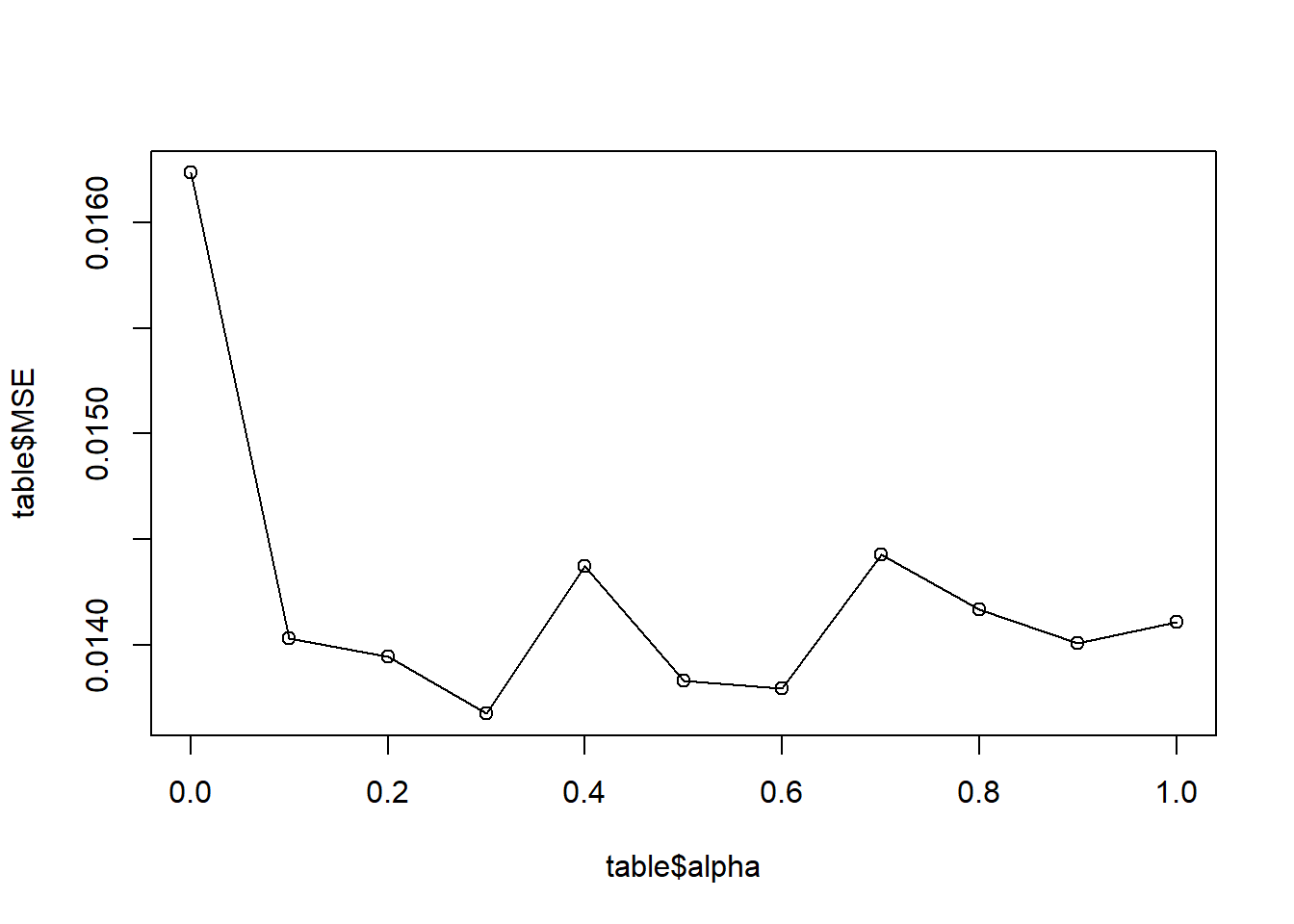
Ridge regression doesn’t cut any variable, but it gives us unique solutions. LASSO estimation can give us a smaller model for the ease of interpretaion. Elastic Net combines Ridge Regression and LASSO, by choosing alpha between 0 and 1. so that it will do feature selection, yet still benefit from Ridge Regression. First, we use the following plot to choose the alpha. The plot describes how mse changes with alpha. However, the plot is random here because mse depends on the split of nfolds. We run it several times and find that mse is always low at alpha=0.9. What’s more, there is no big differences of mse for different alpha, so we stick with it in the following analysis.

#alpha
alpha<- seq(0,1,0.1)
MSE<- seq(0,1,0.1)
table<- data.frame(alpha,MSE)
for(i in 0:10){
  a= i/10
  fit.cv.1<- cv.glmnet(x_train, y_train,alpha=a,nfolds=10)
  table[i+1,2]=min(fit.cv.1$cvm)
}
# plot how mse changes with alpha
plot(table$alpha,table$MSE)
lines(table$alpha,table$MSE)

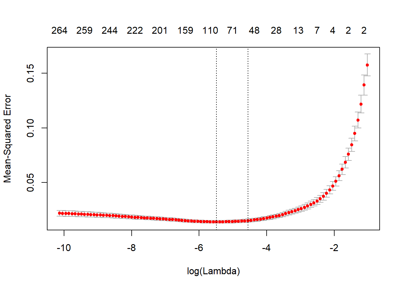
We use cross validation to select the lambda. From this plot we show that as ?? ??? ???, the impact of the shrinkage penalty grows, and the coefficient estimates will approach zero. To have a parsimonious model, we decide to use lambda.1se in our elastic net, which give us 54 variales in our final model. (We also try lambda.min and discuss the results in the appendix.)

fit.fl.cv <- cv.glmnet(x_train, y_train,alpha=0.9, nfolds=10 ) 
plot(fit.fl.cv)

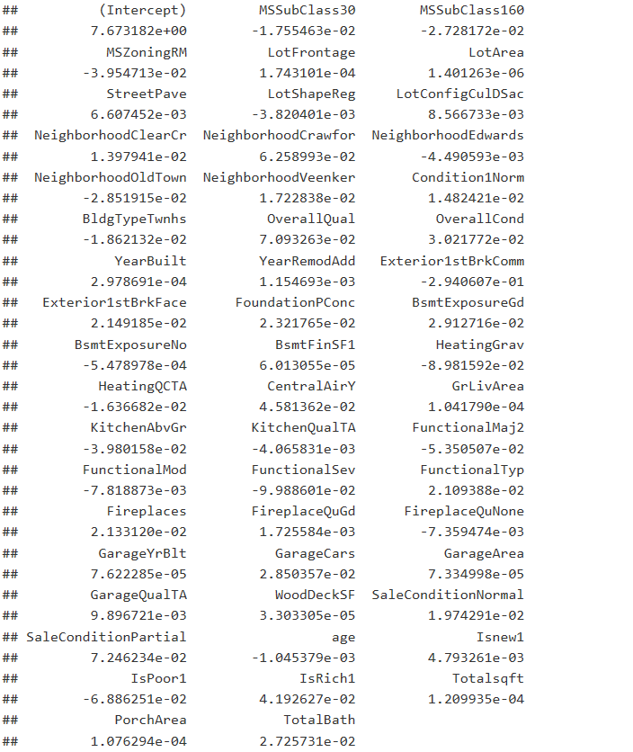
Here are the non-zero coefficients and variables. After cleaning the results and sorting different levels of the same categorical variables, the elastic net returns 41 variables. We conclude that there are six types pf main factors with most effect on home price.

• Area: lot size, shape, and configuration
• Location: neighborhood locations, proximity to main road
• Garage: size, age, quality, and area
• Add-on features: street pave, material, basement, heating or AC, porch area, fireplace
• Age: original construction date, type of dwelling
• Zoning: the building class, the general zoning classification

As a house buyer, it’s easy to notice the relationship between house price and house area, age and locatioin. Since cars are necessary to many families, the condition of garage is also taken into account when chooing houses. However, the majority people may not pay too much attention to add-on features and zoning. From our elastic net results, we can see that these add-on features are also determinants to the house price. It’s not surprising that the quality of heating system, central air condition, and basement are key factors, but house buyer should know that they also pay for the porch area, fireplace, and street pave! Don’t complain the narrow porch while enjoying the lower price of the house. Interestingly, the house in medium density has lower price. The possible reason is that the residental low density represents house and the residental high density represents luxury departments in the downtown, so the prices are both higher than the medium density.

coef.1se <- coef(fit.fl.cv, s="lambda.1se") 
coef.1se <- coef.1se[which(coef.1se !=0),] 
coef.1se
lasso.coef<-data.frame(coef.1se )

The training error of this elastic net is 0.01275193, while the testing error is 0.03670769.

The LASSO estimators are biased, so we use the same set of variables to refit our model using lm() function. The training error of this relaxed elastic net is 0.06878601, while the testing error is 0.01075683.

Neural Net

We also experimented neural net to address this problem. We built a two-layer neural net, used linear ativation function and mean squared error as loss. However, we also acknowledge that the sample size is much limited for a neural net practice.

Model comparison

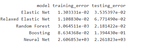
Overall, all the models give us reasonably good results, except for neural net. From this table, we can see that elastic net and random forest give us relatively low training error and testing error. So both models are chosen as our final models.

Conclusion

1. We use elastic net, random forest, boosting and neural net to predict the house price based on internal characteristics, like lot area, material, heating quality, and so on, and external factors, such as zoning, proximity to main road, and so on.
2. We find that the house price mainly depends on six types of factors: Area, Location, Garage, Add-on features, Age and Zoning. It’s easy to notice the relationship between house price and house area, age, locatioin and garage. It’s also not surprising that the quality of heating system, central air condition, and basement are key factors, but house buyer should know that they also pay for the porch area, fireplace, and street pave!
3. All of our models do pretty good job, which means we can predict the house price accurately based on physical characteristics. As we know, homes are hedonic pricing goods through intrinstic features which is all the information used to price the home, while controlling the exterior factors, like sales year fixed effect and local market. So we think the price well captures the information of the houses in this market. Few people in this area treat the house as the investment and hope to make profits by playing the market.
4. Overall, we believe our models work well to predict house price, and they should work better for a healthy housing market.